At Crisp, we help businesses manage all their customer conversations in one place—whether through chat, email, WhatsApp, or other channels - through a help desk platform. As our customers' needs grew, they asked for more detailed insights into their customer support, like response times and team performance.

In the past, we used a MySQL system to calculate these metrics. It worked well but wasn’t enough for users who wanted to explore their data more deeply. They needed more control to analyze and dive into the details (what if we needed response time about VIP customers? Custom SLAs calculation?). Our customers needed something like MixPanel, Posthog, or Amplitude to get an analysis of their conversational data.

With Crisp V4, we’ve built a new system that gives users exactly what they want. But the path wasn't easy.

In this article, we’ll explain why we made this shift, our challenges with MySQL (and why it's not scalable), and how our new ClickHouse-powered engine enables our users to get faster, more detailed insights from their customer data.

Oh, and make sure you read the article until the end! We've added 3 fantastic tips learned from our data storage optimization journey with ClickHouse.

We also share our secret sauce for developing an internal library that wraps the query logic, making analytics requests more accessible and efficient for our API and our dev team.

How our analytics used to work

Around 3,000 000 000 messages are stored, hosted terabytes of conversational data from chat, email, WhatsApp, and more, generating a massive amount of daily information. When we first built our analytics system, finding a database that could handle a massive volume of data while delivering insights quickly and efficiently was a significant challenge.

Back in 2017, there weren’t many database solutions that could scale to meet this need.

To manage this, we chose MySQL and focused on storing only pre-computed metrics, which reduced the data load and made the system scalable.

However, while this approach helped with performance, it limited flexibility and prevented us from offering the deeper, real-time insights that users increasingly demanded.

This pushed us to find a better solution to handle our scale and increasing complexity.

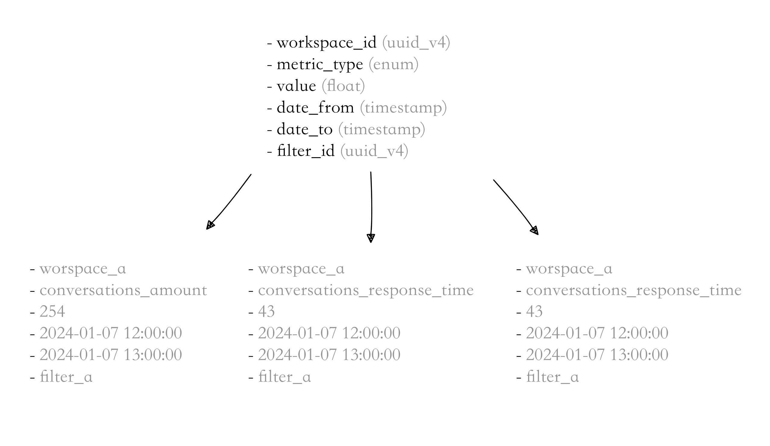
Simplified version of how our MySQL tables looked like

The diagram shows that each workspace had key metrics, such as the total number of conversations, response times, and other performance indicators, pre-calculated and stored in specific tables.

Here’s how it worked:

workspace_id: Each workspace (e.g., a company's Crisp account) had a unique identifier.
metric_type: This defines the stored metric type, such as total conversations or average response time.
value: The actual pre-computed value, like the number of conversations or the average response time.
date_from and date_to: These fields represented the period over which the metric was calculated.
filter_id: A unique filter was applied if users wanted to segment the data (e.g., only viewing data for premium customers).

Getting rid of MySQL: Finding a real-time database that fits terabytes of data

As explained earlier, our users demanded more flexibility and deeper insights from their data, pushing us to look for a more advanced database solution than MySQL. We needed to find a new engine that could overcome these limitations. Here’s what we were looking for in a new system:

Ingest all data without precomputation: We wanted a system capable of handling all raw data, allowing metrics to be computed dynamically in real time. This would give users more flexibility to explore data without being limited to pre-calculated metrics.
Fast filtering: Users must quickly filter data based on specific criteria, such as customer segments or conversation tags. The new engine had to support fast, efficient filtering, even with massive datasets.
Support for fast joins: Many of our users required insights that span across different data tables, such as linking conversations to specific customer details. We needed a system that could handle these joins without slowing down performance.
Update and delete capabilities: The new engine is needed to support real-time updates and deletions. This would allow us to correct or update data as required without reloading the entire dataset, ensuring accuracy and timeliness in our provided metrics.
Efficient data compression: Crisp processes terabytes of conversational data, so efficient data compression was essential. The new engine had to store data in a compressed format to minimize storage costs while maintaining quick query access.

Evaluating ElasticSearch while switching from MySQL

During our search for a new analytics engine, we also evaluated ElasticSearch. While it’s known for its fast search and filtering capabilities, it came with several critical drawbacks that made it inefficient and unsuitable for our needs.

Here’s why ElasticSearch didn’t work for us:

⚠️ High RAM/Heap requirements: ElasticSearch requires a significant amount of RAM and heap memory to function efficiently. As the dataset grows, it demands more memory to store and process indexes, which can quickly become resource-heavy and costly, especially at the scale of terabytes of data.
️⚠️ Massive disk space consumption: ElasticSearch’s data compression is less efficient than we needed. The system consumes a lot of disk space, especially when managing large datasets like Crisp's conversation data. This would have led to skyrocketing storage demands over time, increasing operational costs and making scalability more challenging.
️⚠️ Complex installation and scaling: Setting up ElasticSearch was far more complicated than alternatives. Installing it required a lot of configuration, and adding clusters to scale the system was even more complex. The additional effort and expertise required to maintain and expand an ElasticSearch cluster meant it wasn’t as developer-friendly or quickly manageable for our team.
⚠️ No support for joins: ElasticSearch could not perform joins between different data tables, which was crucial for generating the complex insights our users needed.
⚠️ Inefficient updates/deletes: ElasticSearch also struggled with efficient updates and deletes, which were vital for ensuring the accuracy of our real-time metrics. ElasticSearch supports updates and deletes; however, how it merges segments makes those operations very inefficient, leading to exponential data growth over time, especially when there is a lot of backpressure. ElasticSearch is not made for this.

Evaluating Clickhouse while migrating from MySQL

After evaluating our options, we decided to boot up a ClickHouse cluster on Debian through our hosting provider. Setting it up was incredibly simple—just a matter of running:

curl https://clickhouse.com/ | sh

Within minutes, we had ClickHouse up and running, ready to handle our data. One of the standout advantages of ClickHouse is that it's SQL-compatible, meaning it uses natural SQL syntax, not some custom variation like Cassandra DB does.

This made it easy for our team to get started.

We quickly ran a proof of concept by GPTing table generation and scripting the ingestion of a subset of our raw conversational dataset currently in our MongoDB cluster.

We started with two tables:

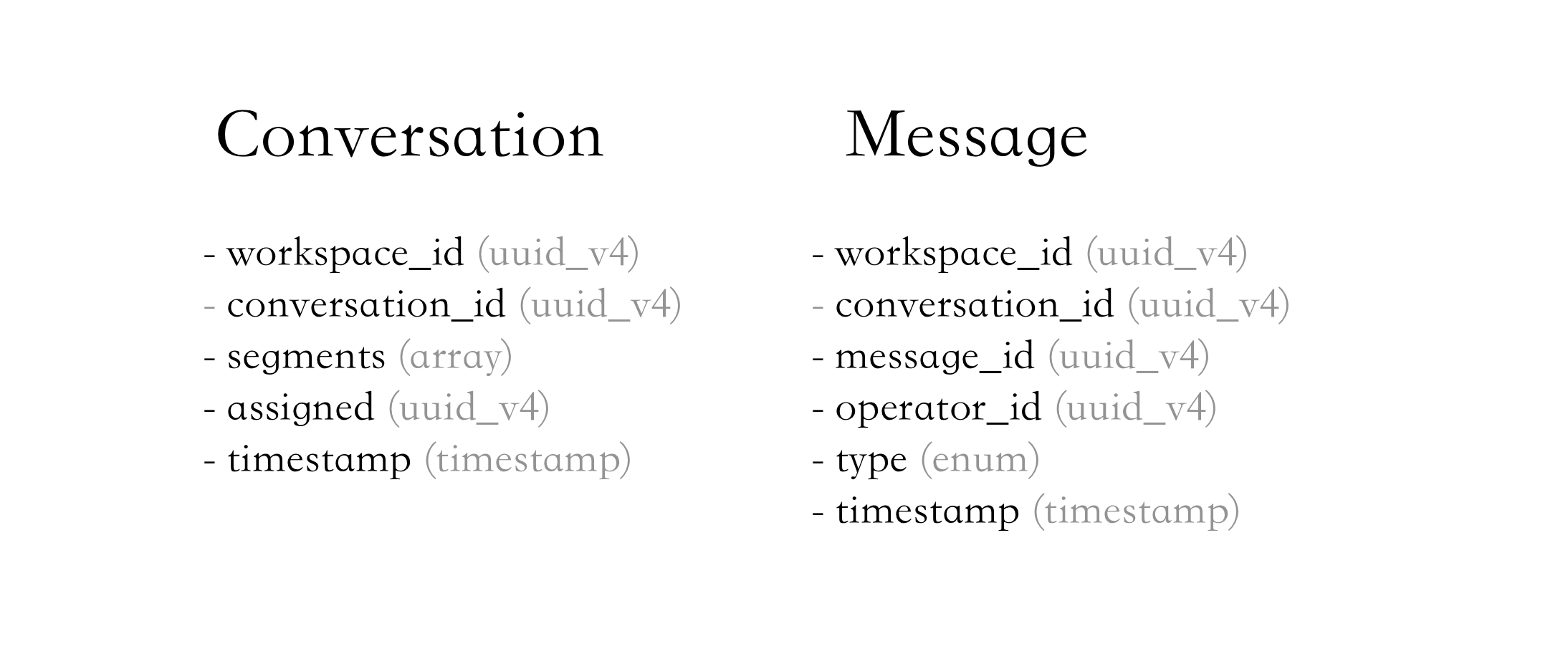
The setup worked right out of the box, and its performance immediately impressed us.

Here’s what blew us away:

😍 Super fast indexing: When we started ingesting data, ClickHouse indexed everything at lightning speed. It can index millions of rows per second. We couldn’t believe how fast it was. In fact, the bottleneck was MongoDB.
😍 Blazing fast queries: Not only was ingestion fast, but querying the data was incredibly quick. The speed with which ClickHouse processed complex queries, even on large datasets, was precisely what we were looking for. Filtering billions of rows and performing joins under the second.
😍 Super efficient data compression: The ingested dataset was over 1.4TB of JSON conversational data. We ended up with around 30GBs
😍 CPU/Memory efficient: Clickhouse is disk-bound, so most operations use SIMD instructions over the disk. RAM usage didn't exceed 500MB, while CPU peaked during the search (however, queries were blazing fast).

ClickHouse immediately showed us that it could easily handle our vast amounts of data, providing the speed and flexibility needed for real-time analytics without any precomputation.

Deep dive into Clickhouse and why it's amazing

So here is a simplified version of our real SQL tables:

CREATE TABLE IF NOT EXISTS conversation
(
  conversation_id UUID,
  workspace_id UUID,
  created_at DateTime,
  updated_at DateTime,
  segments Array(String) CODEC(ZSTD),
  country LowCardinality(Nullable(String)),
  assigned UUID
) ENGINE = ReplacingMergeTree(updated_at)
PARTITION BY (sipHash64(workspace_id) % 16, toYear(created_at))
ORDER BY (workspace_id, conversation_id);

CREATE TABLE IF NOT EXISTS message
(
  conversation_id UUID,
  workspace_id UUID,
  created_at DateTime,
  from LowCardinality(String) CODEC(ZSTD),
  type LowCardinality(String) CODEC(ZSTD),
  origin LowCardinality(String) CODEC(ZSTD),
  operator_id UUID
) ENGINE = MergeTree()
PARTITION BY (sipHash64(workspace_id) % 16, toYear(created_at))
ORDER BY  (workspace_id, conversation_id, created_at);

ClickHouse is a robust database, but it’s crucial to structure your tables correctly to get the best performance. Let’s look at how we’ve set up our tables for Crisp’s analytics needs. Below is a simplified version of our real SQL tables and some key considerations when working with ClickHouse.

The importance of ORDER BY:

In ClickHouse, unlike traditional relational databases, you don’t need primary or foreign keys. The way ClickHouse handles data storage and retrieval is fundamentally different. The most critical aspect is the ORDER BY clause, which defines how the data is stored on disk. The ORDER BY clause plays a crucial role in ensuring that your data is sorted in a way that allows for fast querying and indexing.

For most SaaS platforms, it shall follow this order:

tenant_id
primary_id
timestamp

This setup ensures that the data is ordered and grouped efficiently. By storing the data in this order, ClickHouse can better optimize storage segments, enabling rapid searches and queries over large datasets.

The importance of PARTITION BY:

In ClickHouse, the PARTITION BY clause allows you to control how data is segmented into partitions. However, ClickHouse recommends minimizing custom partitioning unless there’s a strong reason, as automatic data management is usually sufficient.

Click house is not doing any indexing in RAM and is mostly disk-bound so PARTITION BY hints Clickhouse about how indexing and filtering your data.
For instance, in this example from Clickhouse's official documentation:

CREATE TABLE visits
(
    VisitDate Date,
    Hour UInt8,
    ClientID UUID
)
ENGINE = MergeTree()
PARTITION BY toYYYYMM(VisitDate)
ORDER BY Hour;

The data for this table will be broken down and stored on disk in a directory structure like this:

/path/to/clickhouse/data/visits/
└── 2024_01
    ├── data.bin
    ├── primary.idx
    ├── marks.mrk
    └── checksums.txt

When working with large-scale, multi-tenant data in ClickHouse, it’s important to optimize how the data is partitioned and ordered for efficient querying. As mentioned earlier, when you perform a query over a specific year/month using a partition key like toYYYYMM(VisitDate), ClickHouse can quickly locate and filter data because it knows exactly where each partition resides, and the data is pre-ordered.

However, we discovered that ClickHouse is less efficient when performing join operations in a multi-tenant system with the default partition key.

The issue arises because ClickHouse needs to search through multiple partitions, which can slow down queries that require joining data from different tables or segments, especially when dealing with numerous tenants.

The solution: partitioning by sipHash64(workspace_id)

To solve this, we implemented a custom PARTITION BY strategy using sipHash64(workspace_id) % 16, combined with toYear(created_at). This new partitioning approach ensures that tenant data is spread across a limited number of partitions, and the data remains grouped by both the tenant (workspace) and the year. Here's what it looks like:

PARTITION BY (sipHash64(workspace_id) % 16, toYear(created_at))

How this partitioning works

sipHash64(workspace_id) % 16: This hash function spreads tenant data across 16 partitions, ensuring that each partition contains data from multiple tenants but keeps data from a single tenant grouped. When you query using a specific workspace_id, ClickHouse uses the sipHash of that workspace_id to immediately locate which partition contains the data, drastically reducing the number of partitions it needs to scan.
toYear(created_at): In addition to partitioning by tenant, this ensures that data is also split by year, making it efficient to query data for specific time ranges.

Example of structured data

Let’s assume we have the following tenants (workspaces):

workspace_id A
workspace_id B
workspace_id C

And the data spans across different years. After applying sipHash64(workspace_id) % 16, the data might be structured as follows:

/path/to/clickhouse/data/conversations/
└── partition_1
    └── 2023
        └── data for workspace A
    └── 2024
        └── data for workspace B, C
└── partition_2
    └── 2023
        └── data for workspace A
    └── 2024
        └── data for workspace B, C
...
└── partition_16
    └── 2023
        └── data for various workspaces

Each partition (1 through 16) contains data for multiple workspaces, but for any given workspace, the data is always located in one or a few specific partitions. This way, when you perform a query filtering by workspace_id, ClickHouse can immediately determine which partition contains the relevant data and avoid scanning irrelevant partitions.

Benefits of this approach

Reduced filtering overhead: With this partitioning strategy, when you query data for a specific workspace_id, ClickHouse can quickly determine which partition contains the data, minimizing the need for filtering across all partitions. This leads to faster query performance.
Optimized joins: Joins between tables, especially when filtering by tenant (workspace), become much more efficient. Instead of scanning through many different partitions, ClickHouse can focus on a smaller subset of partitions, making join operations faster and more scalable.
Better scalability: Spreading data across 16 partitions ensures that no single partition becomes too large while keeping related data (by tenant and year) in the same partition. This balances the load and keeps the system scalable as the data grows.

The importance of engine:

ClickHouse offers a range of table engines, each optimized for specific use cases, allowing us to handle data ingestion, storage, and querying most efficiently. Picking the right engine is critical for ensuring that your data is stored and processed to meet your needs. Here, we’ll dive deeper into a few key engines—MergeTree, SummingMergeTree, and ReplacingMergeTree—along with examples of their use and a key discovery we made with ReplacingMergeTree.

Caveats:

We recommend adding the following options to your insert queries:

async_insert=1 : The server immediately acknowledges the insert operation and processes it in the background.
wait_for_async_insert=0 : Normally, even with async_insert=1, ClickHouse might still wait briefly for some insert completion or partial data writes. By setting wait_for_async_insert=0, you ensure that the client does not wait at all for any confirmation from the server regarding the insertion status. The insert is fully asynchronous.
async_insert_busy_timeout_ms=60000 and async_insert_use_adaptive_busy_timeout=0: By controlling the timing and behavior of these merges (also known as disk compactions), you can prevent the creation of too many small data segments, which can negatively impact query performance.

The only thing you need is to add this at the end of your INSERT queries:

SET async_insert = 1;
SET wait_for_async_insert = 0;
SET async_insert_busy_timeout_ms = 60000;
SET async_insert_use_adaptive_busy_timeout = 0;

It can also be set globally at the driver level (for instance, when using Python or NodeJS)

1. MergeTree: the versatile workhorse 🐴

The MergeTree engine is the most common and versatile engine in ClickHouse. It allows for data partitioning, indexing, and ordering, making it ideal for large-scale datasets.

Example: Suppose you are storing logs from a web application with fields like timestamp, user_id, and event_type. Using MergeTree, you could set up the table like this:

CREATE TABLE logs
(
    timestamp DateTime,
    user_id UUID,
    event_type String
)
ENGINE = MergeTree()
PARTITION BY toYYYYMM(timestamp)
ORDER BY (user_id, timestamp);

MergeTree is perfect for time-series data, such as log files or monitoring metrics, where fast queries are needed over large datasets ordered by time. However, data won't be deduplicated if you have two keys using the same "PRIMARY KEY" (aka ORDER BY).

2. SummingMergeTree: Perfect for Aggregations

The SummingMergeTree engine is designed to aggregate data. When merging rows, it automatically sums up numeric fields with the same primary key.

Suppose you are storing daily sales data with fields like store_id, date, and sales_amount. Using SummingMergeTree, your table could look like this:

CREATE TABLE daily_sales
(
    store_id UInt32,
    date Date,
    sales_amount Float32
)
ENGINE = SummingMergeTree()
PARTITION BY toYYYYMM(date)
ORDER BY (store_id, date);

Whenever multiple rows for the same store_id and date are merged, the sales_amount will automatically be summed.

Let’s say the following rows are inserted into the table for Store 101:

INSERT INTO daily_sales (store_id, date, sales_amount) VALUES 
(101, '2024-01-01', 1000),
(101, '2024-01-02', 1200);

When you insert additional data:

INSERT INTO daily_sales (store_id, date, sales_amount) VALUES 
(101, '2024-01-01', 500);

The existing row for store 101 will be summed, and this row will look like this:

store_id   date         sales_amount
101        2024-01-01   1500

SummingMergeTree allows us to handle multiple sales records for the same store on the same day, automatically summing them up during the merge process. This is extremely useful for scenarios where new data is constantly being appended and needs to be aggregated efficiently over time.

3. ReplacingMergeTree: handling updates and deduplication

ReplacingMergeTree is used when you need to replace old rows with new ones, making it possible to perform updates on otherwise immutable data. However, one key discovery we made while using ReplacingMergeTree is that you must have a field that changes every time the data is updated. Otherwise, ClickHouse won’t know which version of the row to keep, and deduplication won’t work as expected.

When using ReplacingMergeTree, we discovered that you must include a field that tracks the update timestamp to ensure data is deduplicated correctly. This way, ClickHouse knows which row is the latest when merging. Here’s how we implemented it:

Suppose you have customer data that can be updated frequently, and you want the latest version of each record. Here’s how you’d set up your table with ReplacingMergeTree:

CREATE TABLE customers
(
    customer_id UUID,
    name String,
    email String,
    updated_at DateTime
)
ENGINE = ReplacingMergeTree(updated_at)
PARTITION BY sipHash64(customer_id) % 16
ORDER BY (customer_id);

ReplacingMergeTree(updated_at) ensures that the table keeps the row with the most recent updated_at the field when multiple rows with the same customer_id exist.

Each time a customer record is updated, the updated_at field is refreshed, and when ClickHouse merges the data, it replaces older rows with the latest version based on this timestamp.

Why It's Important? Without the updated_at field (or a similar versioning field), ClickHouse would not know which row to keep, leading to incorrect deduplication and data to grow over time. This field ensures that each record is updated correctly and the latest data is retained.

Bonus: efficient data compression in ClickHouse

One of the standout features of ClickHouse is its ability to efficiently store and compress data, but to truly unlock its potential, you need to carefully structure your data. During our journey with ClickHouse, we discovered several strategies that significantly improved storage efficiency without sacrificing performance. Here are the key findings:

1. ClickHouse is extremely efficient at Storing UUIDs

UUIDs, commonly used for unique identifiers in SaaS applications, can be large in traditional databases. However, ClickHouse excels at compressing and storing UUID data types efficiently. You can store large datasets with UUIDs without worrying about excessive storage overhead.

2. Use LowCardinality(String) wherever possible

If you have columns with repeating values (such as message types, country codes, or other similar categorical data), use LowCardinality(String). While you might be tempted to use ENUM for these fields, LowCardinality performs much more efficient compression without locking you into a fixed set of values.

Let’s say you have a column for message types (e.g., “email,” “chat,” “sms”) or country codes. Instead of using the ENUM type, you can define it as LowCardinality(String), and ClickHouse will handle it with impressive compression and indexing performance.

CREATE TABLE messages
(
    message_id UUID,
    message_type LowCardinality(String),
    country LowCardinality(String)
);

Internally, Clickhouse stores value as integers without worrying about maintaining a schema.

3. Use CODEC(ZSTD) on String Columns

ClickHouse supports various compression codecs, and one of the most efficient is ZSTD (Zstandard), developed by Facebook.

It’s incredibly powerful at compressing string data, making it an excellent choice for columns that store large amounts of text.

What we found: Applying CODEC(ZSTD) to string columns resulted in a major reduction in storage space without any noticeable performance hit on read or write operations.
Example: Here’s how you can apply ZSTD compression to a column:

CREATE TABLE user_messages
(
    user_id UUID,
    message_content String CODEC(ZSTD),
    message_type LowCardinality(String),
    country LowCardinality(String)
);

Why it’s important? ZSTD provides deep compression with very low CPU overhead, making it an excellent option for string-heavy datasets. It helps reduce storage costs while keeping queries fast and efficient.

Creating an internal library to avoid using complex SQL queries

As Crisp's analytics needs grew more complex, we realized that directly writing and managing raw SQL queries became cumbersome and error-prone.

We needed a solution that could simplify and standardize how we request and process analytics data while still maintaining the flexibility to meet evolving business requirements.

This led to the development of an internal library that wraps the query logic, making analytics requests more accessible and more efficient for our API.

Here are the key reasons why we built this internal library:

1. Simplified query management

Writing complex SQL queries repeatedly for every analytics request is not scalable. Each time the logic changes, you must update the SQL in multiple places, leading to inconsistencies and maintenance overhead. By wrapping the query logic in an internal library, we centralized all query operations, making it easier to manage and maintain.

2. Encapsulation of business logic

Our analytics queries often contain specific business logic, such as how metrics are computed, data is filtered, and results are aggregated. Instead of exposing this logic directly to every developer or system that needs it, we encapsulated it inside a library. This ensures that the logic is reusable, consistent, and abstracted from raw SQL, allowing for more accessible updates and scaling.

3. Flexibility with a JSON Schema

To make it easier for our API to request different kinds of analytics data, we introduced a JSON schema format that abstracts away the complexity of SQL.

Instead of constructing SQL queries manually, our API can pass a structured JSON request that the internal library interprets, constructs the necessary queries, and returns the result.

4. SQL query generation with Knex

We have chosen Knex.js, a flexible SQL query builder for Node.js, to handle the underlying query construction. Knex allows us to write database-agnostic queries in JavaScript, which makes it easier to work with complex queries and generate Common Table Expressions (CTEs), joins, and other advanced SQL constructs without writing raw SQL. It also supports dynamic query building, making it a perfect fit for our JSON schema-driven approach.

Why Knex?

Database-Agnostic: Knex is database-agnostic, meaning the same code can work with different databases, making it a future-proof choice.
CTE and Advanced Query Support: Knex provides full support for advanced SQL features like Common Table Expressions (CTEs), which we use extensively for modular, reusable queries.
Dynamic Query Construction: With Knex, we can dynamically construct queries based on the incoming JSON request. For example, we can conditionally add filters, groupings, and aggregations depending on the parameters specified in the request.
Readable and Maintainable: Unlike raw SQL, Knex allows us to write queries in a more readable, JavaScript-friendly way, which integrates well with the rest of our codebase.

JSON schema example for analytics requests

We designed a JSON schema to standardize how analytics queries are requested. This schema allows our API to specify the type of metric, how to split the data (e.g., by country, segment), and any filtering criteria. Here’s a simplified example of how an analytics request might look:

{
  "metric": "conversation",
  "type": "response_time",
  "split_by": "country",
  "date": {
    "split": "all",
    "timezone": "Europe/Vienna",
    "to": "2024-08-27",
    "from": "2023-08-28"
  },
  "filter": {
    "segment": {
      "include": ["vip"],
      "exclude": ["bug"]
    }
  }
}

Chaining CTEs for modular query construction

One of the challenges we faced was dealing with requests that required multiple layers of filtering, aggregation, and transformations before arriving at the final result. For example, one common analytics request involved calculating conversation response times, split by country, and filtered by user segments. This is where the use of CTEs proved invaluable.

Rather than writing a single, massive SQL query that handled all of this logic in one go, we broke the process down into smaller, manageable steps, each encapsulated in its own CTE. Each CTE was responsible for a specific stage of the query:

Date filtering: The first step involved filtering conversations based on a provided date range and converting timestamps to the appropriate timezone. This CTE allowed us to isolate the date logic, making it easy to modify or reuse elsewhere.
Segment filtering: Next, we applied filters for user segments, such as including only VIP customers and excluding those marked as "bugs." This was layered on top of the date-filtered data from the previous CTE.
Response time calculation: We calculated response times using the filtered data by joining the filtered conversation data with the message table to determine the time between the first customer message and the first operator response. By encapsulating this logic in its own CTE, we kept the calculation clean and easily testable.
Final aggregation: The final step was to aggregate the response times by country and calculate averages. This involved grouping the data by country, ensuring the result was broken down as needed for reporting.

By chaining these CTEs together, we not only simplified but also made query generation modular. Each step was independently manageable, reusable, and easy to debug, which became critical as the complexity of the requests increased.

Here’s a simplified version of how we chained CTEs to generate a query for calculating conversation response times, split by country and filtered by user segments, using Knex.

Step 1: Date Filtering CTE

The first CTE filters the conversations based on the date range provided in the request, adjusting for timezone.

function dateFilterCTE(knex, request) {
  return knex
    .select('conversation_id', 'created_at', 'country', 'segment')
    .from('conversation')
    .whereBetween('created_at', [
      knex.raw(`toDateTime(?, ?)`, [request.date.from, request.date.timezone]),
      knex.raw(`toDateTime(?, ?)`, [request.date.to, request.date.timezone])
    ]);
}

This CTE extracts the relevant columns (conversation_id, created_at, country, and segment) from the conversation table, apply a date range filter based on the from and to dates, converted to the appropriate timezone.

Step 2: Segment Filtering CTE

The next step is to filter the data based on the segments provided in the request (e.g., include "VIP" customers and exclude those marked as "bug"). This CTE chains on top of the date-filtered CTE.

function segmentFilterCTE(knex, request, baseQuery) {
  let query = baseQuery;

  if (request.filter && request.filter.segment) {
    if (request.filter.segment.include) {
      query = query.whereIn('segment', request.filter.segment.include);
    }
    if (request.filter.segment.exclude) {
      query = query.whereNotIn('segment', request.filter.segment.exclude);
    }
  }

  return query;
}

This CTE further filters the conversations by including or excluding certain customer segments based on the request parameters.

Step 3: Response Time Calculation CTE

With the filtered conversations from the previous steps, we now calculate the response time for each conversation. This involves joining the filtered conversations with the message table to calculate the difference between the first customer message and the first operator response.

function responseTimeCTE(knex, baseQuery) {
  return knex
    .with('filtered_conversations', baseQuery)
    .select('conversation_id', 'country', 'segment')
    .select(
      knex.raw('MIN(operator_message.created_at) - MIN(user_message.created_at) AS response_time')
    )
    .from('filtered_conversations')
    .join('message AS user_message', function () {
      this.on('filtered_conversations.conversation_id', '=', 'user_message.conversation_id')
        .andOn('user_message.from', '=', knex.raw('?', ['user']));
    })
    .join('message AS operator_message', function () {
      this.on('filtered_conversations.conversation_id', '=', 'operator_message.conversation_id')
        .andOn('operator_message.from', '=', knex.raw('?', ['operator']))
        .andOn('operator_message.created_at', '>', 'user_message.created_at');
    })
    .groupBy('conversation_id', 'country', 'segment');
}

This CTE calculates the response time by finding the difference between the created_at timestamp of the first operator message and the first user message. It groups the result by conversation_id, country, and segment.

Step 4: final aggregation query

Finally, we aggregate the results by country and calculate the average response time for each country.

function buildConversationResponseTimeQuery(knex, request) {
  // Step 1: Date Filter CTE
  const dateFilteredCTE = dateFilterCTE(knex, request);

  // Step 2: Segment Filter CTE
  const segmentFilteredCTE = segmentFilterCTE(knex, request, dateFilteredCTE);

  // Step 3: Response Time CTE
  const responseTimeCTEQuery = responseTimeCTE(knex, segmentFilteredCTE);

  // Step 4: Final Query - Group by Country and Calculate Average Response Time
  return knex
    .with('response_times', responseTimeCTEQuery)
    .select('country')
    .avg('response_time as avg_response_time')
    .from('response_times')
    .groupBy('country');
}

This final query:

Chains the CTEs together, starting from date filtering, segment filtering, and response time calculation.
Uses the final response time CTE as a clause.
Groups the results by country and calculates the average response time.

Running the Query

Here’s how we can execute the query using Knex:

const knex = require('knex')({ client: 'clickhouse' });

const request = {
  metric: "conversation",
  type: "response_time",
  split_by: "country",
  date: {
    split: "all",
    timezone: "Europe/Vienna",
    to: "2024-08-27",
    from: "2023-08-28"
  },
  filter: {
    segment: {
      include: ["vip"],
      exclude: ["bug"]
    }
  }
};

const query = buildConversationResponseTimeQuery(knex, request);

query.then(result => {
  console.log(result);
}).catch(error => {
  console.error(error);
});

Last step: building a great user interface

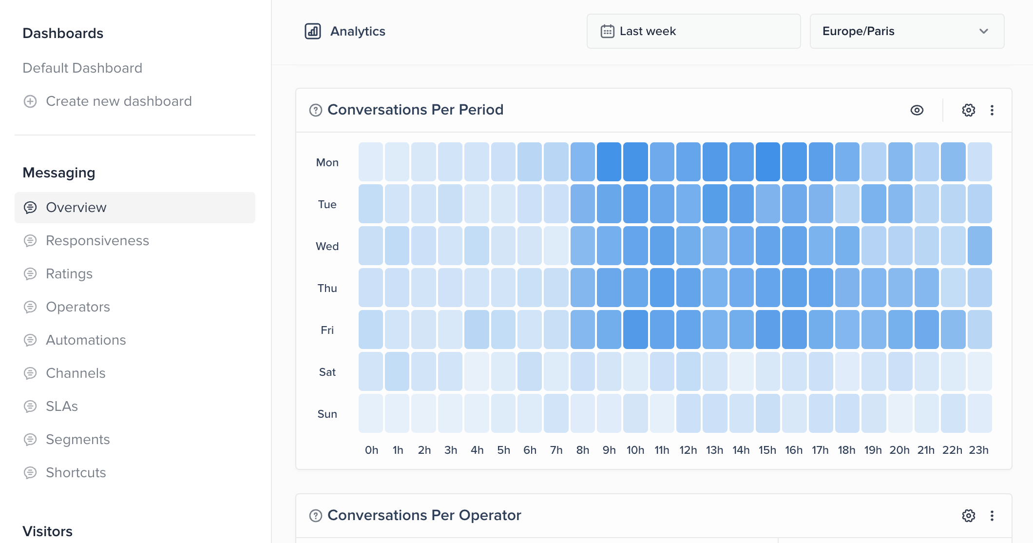
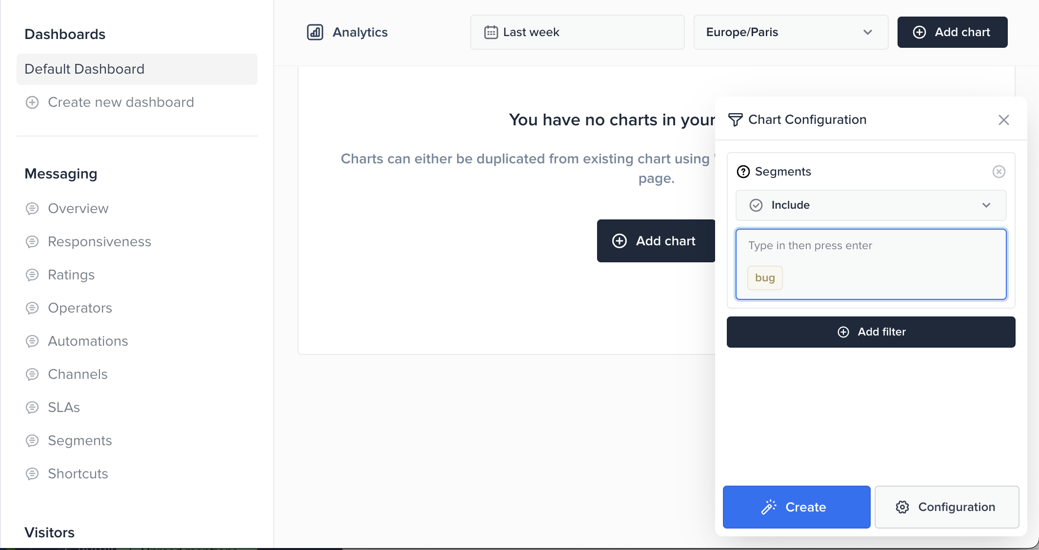
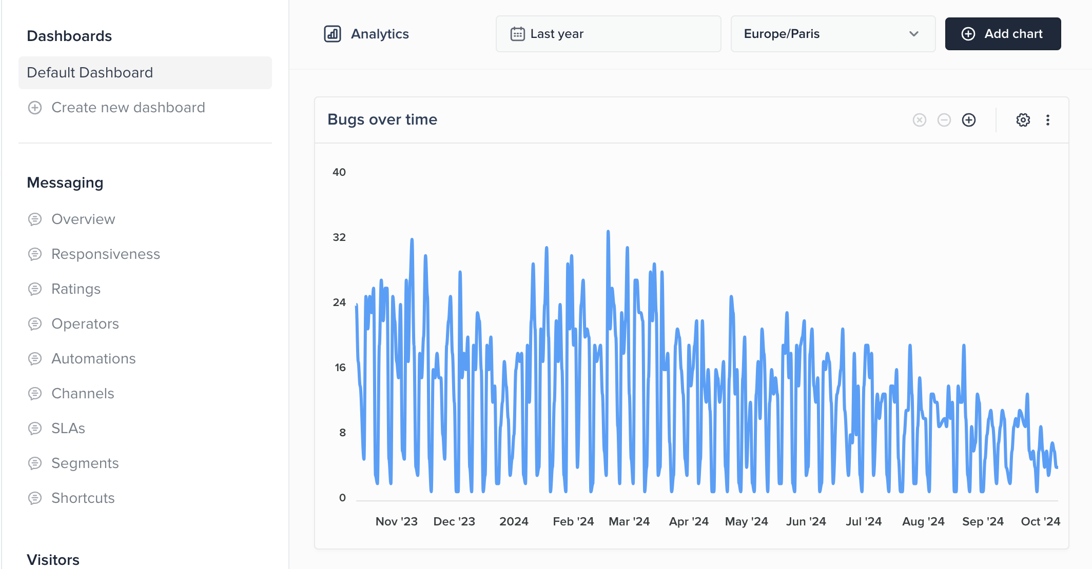
With our modular system in place, we developed a powerful and flexible analytics platform that enables users to perform various calculations. The beauty of this system is its generic structure, which supports multiple metrics and breakdowns, allowing users to customize their queries without needing to know the underlying complexities of the data.

By integrating this with a user-friendly UI, we empowered users to:

Create their own metrics: Users can easily define and build metrics through an intuitive interface, selecting the relevant filters, date ranges, and data splits.
Playground for experimentation: The UI acts as a playground where users can experiment with different filters and visualizations to gain deeper insights into their data without technical barriers.

This combination of a modular backend system and a versatile frontend UI has resulted in a highly adaptable and powerful analytics solution, making it easy for users to extract meaningful insights in real-time.

Conclusion

Building a robust analytics system capable of handling terabytes of data is no small feat, but it's a challenge we successfully tackled at Crisp. Our journey from MySQL to ClickHouse demonstrates the power of choosing the right tools and strategies when scaling data analytics for a SaaS platform.

Key takeaways from our experience include:

The importance of selecting a database that can handle large-scale, real-time analytics without sacrificing performance or flexibility.
How ClickHouse's efficient data compression and storage capabilities significantly reduced our infrastructure costs while improving query speeds.
The value of thoughtful table design, including strategic use of partitioning, ordering, and compression techniques to optimize performance.
The benefits of building an internal library to abstract complex SQL queries make it easier for our API to request and process analytics data.
The power of using Common Table Expressions (CTEs) and a query builder like Knex.js to create modular, maintainable, and flexible query logic.
The importance of a user-friendly UI that empowers users to create custom metrics and experiment with data analysis without needing technical expertise.

By sharing our experiences and the lessons we've learned, we hope to provide valuable insights for other companies facing similar challenges in building scalable analytics systems. As data grows exponentially in the SaaS world, having a robust, efficient, and flexible analytics engine becomes increasingly crucial for delivering actionable insights to users.

This story is part of the Crisp v4 release; to see the full story, check it out here: https://crisp.chat/en/v4/.

From Zero to Terabytes: Building SaaS Analytics with ClickHouse